The need to develop treatments and/or programs specific to a disease requires the analysis of outcomes to be specific to that disease. Such endpoints as heart failure, death due to a specific disease, or control of local disease in cancer may become impossible to observe due to a prior occurrence of a different type of event (such as death from another cause). The event which hinders or changes the possibility of observing the event of interest is called a competing risk.
The usual techniques for time-to-event analysis applied in the presence of competing risks give biased or uninterpretable results. The estimation of the probability of the event therefore needs to be calculated using specific techniques such as the cumulative incidence function introduced by Kalbfleisch and Prentice. The model introduced by Fine and Gray can be applied to test a covariate when competing risks are present. Using specific techniques for the analysis of competing risks will ensure that the results are unbiased and can be correctly interpreted.
Keywords
.
INTRODUCTIONCompeting risks (CR) has been recognized as a special case of time-to-event analysis since the 18th century. Occasionally work in the statistical or mathematical area has been published incorporating new developments, including the monograph of David and Moeschberger.1 As the data became more extensive, clear, and precise regarding the different types of outcomes, CR resurfaced as a crucial type of analysis within time-to-event analysis, necessary for a better understanding of a disease. The connection between the mathematical results and the applied field needed to be made. Several authors have contributed to the understanding of CR situations.2, 3 Other authors enhanced and developed techniques and in some cases made available ready-to-use computer code for applied statistics.4, 5, 6
INTRODUCTION TO TIME-TO-EVENT ANALYSISIn many studies the outcome is observed longitudinally. In this way every subject in the cohort is observed for a period of time until the event occurs. For example the event of interest may be death, heart attack, or cancer recurrence. The goals of the study may be to estimate the probability of the event occurrence or its association with covariates of interest like treatment or subject characteristics. The statistical analysis employed is called time-to-event analysis or sometimes survival analysis. The most common method to estimate the probability of an event is a nonparametric approach customarily called the Kaplan-Meier7 (KM) or product limit method. The main assumption of the KM estimation for survival is that the censored observations will experience the event if followed long enough.
For the rest of this paper, the probabilities for the event will be given rather than the probability for free-of-event. For example, instead of probability of survival, probability of death will be presented, which can be estimated using the complement of the KM estimator: 1-KM.
INTRODUCTION TO COMPETING RISKSIt is not uncommon for a participant in a study to experience more than one type of event. A CR situation happens when the occurrence of one type of event changes the ability to observe the event of interest. Miyasaka et al.8 conducted a study on a community-based cohort of patients diagnosed with atrial fibrillation between 1986 and 2000 in Olmsted County, Minnesota, United States. The primary outcome was the onset of dementia. The median follow-up was 4.6 years. Other types of events were stroke and death. Of the 2837 individuals with atrial fibrillation, 299 had dementia and 1638 died by the time of the analysis. The numbers with stroke are not reported and are censored in the analysis. The conclusion of the study was that the incidence of dementia among the individuals with atrial fibrillation is common (10.5% at 5 years using KM method). The occurrence of stroke before dementia does not affect the observation of dementia and thus it is not a CR event. For the sake of argument we ignore the fact that multiple strokes can cause dementia. On the other hand, a death without prior dementia makes the observation of dementia impossible. Therefore, a death without dementia is a CR event for the endpoint of dementia. Also a severe head injury might be considered a CR event since the behavioral changes of the patient might make the diagnosis of dementia impossible.
A more subtle CR situation occurs in the study conducted by Whalley et al.9 of the importance of echocardiography. This cohort of 228 elderly symptomatic patients underwent echocardiography and was followed for either cardiovascular hospitalization or cardiovascular death. The hypothesis was that the echocardiography features predict for cardiovascular event. The main outcome was defined as the composite measure including cardiovascular death and/or hospitalization. For this type of outcome a death due to causes other than cardiovascular disease is a CR event and, as such, a patient is no longer at risk of having any of the events of interest.
A 3-arm, double-blind, randomized trial was conducted spanning 931 centers and 24 countries to test the effect of valsartan vs valsartan+captopril vs captopril alone (VALIANT)10 on all-cause mortality. In total, 14 703 post-myocardial infarction patients with left ventricle dysfunction and/or heart failure accrued 1:1:1 in the 3 arms. Since any death was considered an event, this type of outcome does not have CR. The study supported the hypothesis that survival in the 3 arms was different. However, gastrointestinal (GI) bleeding was identified as a serious side effect in all 3 arms. Moukarbel et al.11 studied the possible factors which could predict GI bleeding. For this endpoint, death without GI bleeding is a clear CR.
An increasing number of researchers recognize the presence of CR and the need for proper techniques to be applied. A cohort of 972 patients with non-ST-segment elevation acute coronary syndrome between 2001 and 2005 was studied by Núñez et al.12 One of the goals of the study was to find factors associated with rehospitalization for acute heart failure. Among the factors studied were diabetes, previous history of ischemic heart disease, chronic kidney failure, smoking history, and treatment history. The authors recognized the possibility of CR such as death before rehospitalization and correctly applied specific techniques to account for the CR situation.
Melberg et al.13 studied a cohort of 1234 patients with symptomatic coronary artery disease who received 2 types of treatments: coronary artery bypass grafting (n=594) or percutaneous coronary intervention (n=640). Of the 301 deaths observed during the follow-up, 42.5% were cardiac deaths and the rest were noncardiac deaths. The authors present results for all-cause mortality as well as for cardiac mortality and noncardiac mortality. They point out that the percentage for all-cause mortality is the sum of the percentage of cardiac and noncardiac mortality correctly estimated taking into account the CR. The authors emphasize the importance of analyzing each of the events of interest rather than combining them into an overall mortality. This topic is also expounded at a more general level by Mell and Jeong.14
As could be surmised from the above examples, the main question when CR are present is whether to ignore the CR and censor the observations involving CR or to account for CR. When the CR are ignored and the CR observations are censored the analysis reduces to a “usual” time-to-event scenario. Due to the familiarity of this type of analysis and the availability of software, many researchers resort to this approach, as seen in the earlier examples. However, it is unanimously agreed not only among statisticians2, 15, 16, 17, 18 that the estimation of the probability of event in this case overestimates the true probability. The next natural question is whether the modeling can be performed within these bounds (ignoring/censoring CR). This is more ambiguous and more difficult to grasp. While such an analysis may not be without value its interpretation is almost always fraught with difficulties. The main requirement is that the CR event (whose observations were censored and mixed with the true censored observations) needs to be independent of the event of interest. If this is the case, then the results could be interpreted as the effect of covariates when the CR events did not exist. However, this assumption cannot usually be made and cannot be verified or tested. In conclusion, every time the CR observations are censored the estimation of the probability of event is incorrect and the interpretation of the effect of covariates is not clear due to the lack of knowledge of the independence between the event of interest and CR event.
When the analysis is performed accounting for CR (and coded distinctly from the event of interest or the censoring) then the probability is correctly estimated and the modeling has a straightforward interpretation. There is no assumption of independence to hinder the interpretation. The coefficient of a covariate thus estimated represents the effect of that covariate on the observed probabilities.
Several authors19, 20 attempted to compare the two approaches in terms of the power of the tests using simulations. However, the researcher needs to be aware that the main problem is in the interpretation of the results. Regardless of how powerful the tests are, the analysis needs to answer the question of the study.
ESTIMATING THE PROBABILITY OF EVENTIt is common practice to apply the KM method to estimate the probability of an event. The typical formula for the KM estimate is

This formula can be transformed through algebraic manipulation to express the probability of event as:

In the presence of CR there are at least 2 types of events: event of interest, identified with the subscript e, and the competing risk event, identified with the subscript c. Kalbfleisch and Prentice introduced the formula for the probability of an event of interest in the presence of CR:

It is interesting to note the relationship between (1) and (2). Since di is the number of all events at ti, it can be conceived as the sum of the number of events of interest dei and the number of CR events dci at time ti. As such, the probability of any type of event can be decomposed as:

Thus the probability of all events can be decomposed in the probabilities for each type of event.
If 1-KM is used to calculate the probability of an event of interest in the presence of CR, survival of all events in formula (2) is replaced by the KM estimate based on the events of interest only. This will bias the results, as will be shown later. The main assumption for the use of the KM method is that the censored patients, if followed long enough, will eventually experience the event. However, when the KM method is used in the presence of CR, the patients experiencing types of events other than the event of interest are usually censored, even though they are no longer at risk for the event of interest. Furthermore, the nice decomposition seen in (3) cannot be performed for the 1-KM formula.
In applied situations it is possible that there are several other types of events which are not of interest. In this case all can be grouped under the umbrella of CR events.
It will be shown through an example that the use of the KM method is not appropriate in the presence of CR.
Description of the ExampleA dataset collected to study the late effects of the treatment for Hodgkin lymphoma will be used for illustration. The main outcome is hospitalization for cardiac disease. The Hodgkin lymphoma is a type of cancer which appears mostly in young adults. In its early stages it is almost curable, with 10-year overall survival of 70%. Thus, a cohort of these patients is ideal to study the long-term side effects of treatment. The dataset used here is a subset of a larger cohort which will be reported elsewhere. The data are also modified to serve our purposes. For example, for simplicity, we kept in the data only patients who had either chemotherapy or radiation, excluding those with combined treatment. To increase the rate of CR (death without cardiac hospitalization), we included patients of all stages. Some follow-up and death dates were imputed. Due to the modifications that were made to the data, no clinical conclusions can be drawn from this analysis. The data presented here reference 689 records with 93 cardiac hospitalizations and 467 deaths.
The rates for cardiac hospitalization and for death without a cardiac event will be calculated using both the KM method (1) and the cumulative incidence function (CIF) introduced by Kalbfleisch and Prentice21 for this purpose (2).
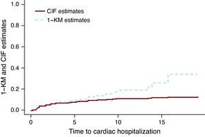
The Kaplan-Meier Method Applied to a Competing Risks Situation Overestimates the True Rate of the EventFigure 1 presents the CIF and 1-KM estimates for cardiac hospitalization of the group treated with chemotherapy only. The broken line corresponding to the 1-KM estimates is above the solid line representing the CIF estimates. It can be shown mathematically that 1-KM always overestimates the probability of event. A common misconception is that 1-KM estimates are correct if the two events are independent. The independence between events is always questionable at best, but even when the data is simulated as independent events, the difference between the CIF estimates and the 1-KM exists. The size of the difference depends on the number of events, both for events of interest and the CR events. In Miyasaka et al.,8 the incidence of dementia at 5 years using the KM method was 10.5%. The number of CR (deaths) was about three quarters of the total number of events, which suggests that their estimate may be much larger than what is observed.

Figure 1. Cumulative incidence function vs 1- Kaplan-Meier estimates.. CIF, cumulative incidence function; KM, Kaplan-Meier.
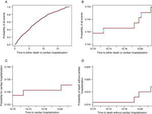
The Cumulative Incidence Function Partitions the Probability of Any Event (Cardiac Hospitalization or Death) Into the Constituent ProbabilitiesAlgebraically this is proven in (3). However, for a deeper understanding of how it works, it will be shown graphically that from the probability of all events a portion participates to the CIF for one event and the other to the CIF for the other event. Figure 2A shows the probability of any event: cardiac hospitalization or death without cardiac hospitalization. Figure 2B contains only the curve between 10.7 and 10.85 years, such that the steps are visible. On each step there is a circle. The open circles appear on the steps in which a death was observed while the solid circles are on the steps in which a cardiac hospitalization occurred. The steps with solid circles participate in the CIF for the cardiac hospitalization in panel C and the ones with open circles participate in the curve for death in Figure 2D. Thus, each step will contribute to the probability of the event which causes it. In this way, at any point in time the probability of all events is the sum of the probability of the event of interest and the probability of CR. Note that the last 3 panels (Figure 2B-D) show the same window of time and have the same length for the y-axis such that the size of the steps can be compared between them. Table 1 shows these probabilities at 1, 2, 3, 4 and 5 years.

Figure 2. The partition of the probability of all events into the constituent probabilities. A. The probability of cardiac hospitalization or death. B. The probability of cardiac hospitalization or death only for the window of time 10.70 - 10.85 years. The solid circles indicate the cardiac hospitalization and the open circles represent deaths without cardiac hospitalization. C. The probability of cardiac hospitalization in the window of time 10.70 -10.85 years. D. The probability of death without cardiac hospitalization in the window of time 10.70-10.85.
Table 1. The Probability for Any Event Is the Sum of the Constituent Probabilities.
| Year of reporting | Probability of cardiac hospitalization | Probability of death | Probability of either cardiac hospitalization or death |
| 1 | 0.038 | 0.054 | 0.092 |
| 2 | 0.054 | 0.139 | 0.193 |
| 3 | 0.072 | 0.193 | 0.265 |
| 4 | 0.076 | 0.25 | 0.327 |
| 5 | 0.087 | 0.305 | 0.392 |
Because the 1-KM overestimates the probability for an event, if we tried to add the 1-KM estimates for cardiac hospitalization to the 1-KM for death we would obtain a much higher rate than the probability of any event. In some cases the number obtained is even larger than 1, which proves that in the presence of CR, 1-KM estimates are not even probabilities.
Does the Cumulative Incidence Function Method Indeed Estimate the Correct Probability of Event?For this purpose a dataset of 500 records was simulated such that there is no censoring before 5 years and there are 2 types of events: type 1and 2. Table 2 shows for each type of event the number observed up to that point in time, the crude rate, and the CIF estimate, which are exactly equal. Equality happens only when there are no censored observations up to that point in time. In the presence of censored observations within the reported years the equality does not hold and the correct way to estimate the probability is the CIF and not the crude rate.
Table 2. The Probability of the Two Types of Event When There Are No Censored Observations Up to 5 Years.
| Year of reporting | Number of type 1 event | Crude rate of type 1 event (%) | CIF for type 1 event (%) | Number of type 2 event | Crude rate of type 2 event (%) | CIF for type 2 event (%) |
| 1 year | 31 | 6.2 | 6.2 | 39 | 7.8 | 7.8 |
| 2 years | 49 | 9.8 | 9.8 | 74 | 14.8 | 14.8 |
| 3 years | 62 | 12.4 | 12.4 | 105 | 21 | 21 |
| 4 years | 76 | 15.2 | 15.2 | 140 | 28 | 28 |
| 5 years | 87 | 17.4 | 17.4 | 170 | 34 | 34 |
CIF, cumulative incidence function.
In conclusion, to calculate the probability of event in the presence of CR one has to use the method introduced by Kalbfleisch and Prentice, customarily called the cumulative incidence curve.
MODELINGAn important aspect in an analysis is to test the association between a covariate and the event of interest, either alone or adjusting for other factors. In the absence of CR this is routinely accomplished by using the Cox proportional hazards (Cox PH) model.22
In the presence of CR, the Cox PH model does not have a simple interpretation. If the time to the 2 types of events can be considered independent, then the results can be interpreted as showing the effect in the situation when CR do not exist. However, the assumption of independence can rarely be made or tested and thus the results from Cox PH model are usually not interpretable.
Fine and Gray ModelFine and Gray6 (F&G) modified the Cox PH model to allow for the presence of CR. The technical modification consists of keeping the CR observations in the risk set with a diminishing weight. In this way the F&G method models the subdistribution hazards. The effect estimated using the F&G model shows the current and real differences between the treatment groups in terms of subdistribution hazards ratios. The assumption of proportionality of hazards is still a requirement, but of course it refers to the subdistribution hazards. The F&G model can accommodate time dependent coefficients to model the nonproportionality of hazards. This model can be applied to both the event of interest (cardiac hospitalization) or the CR (death).
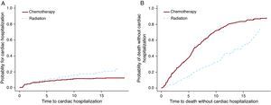
The Cox PH and F&G models were applied to the Hodgkin lymphoma dataset to test the treatment option of chemotherapy vs radiation. For this example (Table 3) the results from the Cox PH and the F&G models differ substantially (first 2 rows). As mentioned above, the Cox PH results are not interpretable and cannot be used. The second row shows that there are more cardiac hospitalizations among the radiation group and the third row shows more deaths among the chemotherapy group. Figure 3 shows these results graphically. It is possible that chemotherapy alone was given to patients with more advanced disease, and these patients were also more likely to die of their cancer. On the other hand radiation alone was probably given to patients at an early stage who lived longer after the Hodgkin lymphoma diagnosis. These patients had more of a chance to develop late side effects like cardiac disease.
Table 3. The Effect of the Treatment When Cox Proportional Hazards and Fine and Gray Models Are Employed.
| Endpoint | Model | HR | 95% CI for HR | P-value |
| Cardiac hospitalization | Cox PH | 1.07 | 0.71-1.63 | .74 |
| Cardiac hospitalization | F&G | 1.63 | 1.1-2.445 | .02 |
| Death without cardiac hospitalization | F&G | 0.38 | 0.31-0.47 | <.0001 |
CI, confidence interval; Cox PH, Cox proportional hazards model; F&G, Fine and Gray model; HR, hazard ratio.
The hazard ratios show the increase of the hazards for the radiation group as compared to chemotherapy group.

Figure 3. The effect of the treatment for cardiac hospitalization and for death.
As can be seen from this example, the interpretation of results is a work of collaboration between the statistician and the clinician who has a thorough knowledge of the disease.
The presence of CR complicates both the analysis and the interpretation of data. To allow the reader to correctly interpret the results, the authors need to include details on the observed events even though they may not seem important at first sight. Therefore, when the endpoint is observed over time the authors need to include the event of interest, whether there is the possibility of CR, how many patients experience any of these types of events, and the duration of follow-up. In the presence of CR it is informative to include the analysis for the event of interest as well as the analysis for CR, as they complement each other and could help interpret the results.
The Logistic ApproachLet us suppose first that we are in the framework of no CR. When the outcome is expected to occur within a short interval (eg, 1 year), the tool of choice for many researchers is logistic regression. This is appropriate if every individual in the cohort has the minimum follow-up, in this case 1 year. In fact the estimate for 1-year mortality will coincide with the estimate of 1-KM. The temporal cut-off point needs to be the same for every individual in the cohort. Therefore, if the outcome of interest is 1-year mortality and 1 individual in the cohort dies at 1 year and 2 days, that person should be considered as “no event at 1 year.” This may reduce the number of events, which translates into a less than ideal analysis when many observed events occur after the cut-off point.
The same basic rules apply when CR are present. All individuals in the cohort must have the minimum follow-up chosen as the time cut-off point, and that cut-off point must apply for everyone in the cohort. The coefficients and p-values will in general give the same message but will not be exactly the same for the logistic regression as compared to F&G model. First of all, in logistic regression the coefficient represents the log of the odds ratio, while in F&G model it is the log of the ratio of the hazards subdistributions. In addition, in logistic analysis not all events are used and of course a different model is used.
POWER CALCULATIONWhen the measure is time-to-event, the power calculation has two stages. The first step is to calculate the number of events needed in order to detect a specific effect size. Next, the number of patients needed to observe that number of events is calculated. It was emphasized in the previous sections that when CR are present it is not possible to observe all the events of interest due to the occurrence of CR. Since the number of events is central in the calculation of power, extra care needs to be taken to ensure that CR are taken into account. If the CR are not considered, then the study will be underpowered and therefore likely unsuccessful (and possibly unethical).
SOFTWAREThe open source R software on CRAN (the Comprehensive R Archive Network) site (http://cran.r-project.org/) offers a package (cmprsk) implemented by Dr. Robert Gray containing the necessary tools for a complete analysis accounting for CR. Thus, one could obtain observed probability plots for the event of interest and a p-value based on Gray's test, which is a modified logrank test for CR situation. Within the package there is also a function for modeling using the F&G approach. Luca Scruca enhanced the output delivery of the modeling function for an easier read by incorporating in the package a summary type function. The model has the possibility to check the proportionality of hazards, and terms for time dependent coefficients can be included. The code cannot accommodate left truncation or cluster data. The left truncation would be useful for the analysis of multiple/recurrent events per patient or for the analysis of case cohort. A code for case-cohort studies was developed (Pintilie et al.23) and can be obtained from the authors. Zhou et al.24 extended the F&G model to accommodate stratified data and will also have a version for cluster data. At this point the code may be obtained from the authors for both cases but it is likely that it will be submitted to CRAN.
STATA 11 has recently implemented the F&G model. One needs to be aware that the graphs obtained using STATA are predictive rather than observed probability graphs. There are two caveats when predicted curves are used: a) the lines will always appear as if the proportionality of hazards is satisfied, and b) the number of steps in each curve will be larger than the number of events in each subgroup, giving the impression that there are more events than there really are.
CONCLUSIONSThe availability of large datasets with complete follow-up for several endpoints is continuously increasing. There is also an increasing need for analyses which are concerned with a precise endpoint like death from heart failure or disease control or control of local disease. All these endpoints could potentially have CR. Therefore it is essential that the CR be considered from the design stage to the interpretation of results. While the Cox PH model may have a limited value when independence is considered, the KM estimates are not correct and cannot be interpreted. Thus, specific techniques like CIF and F&G models made available in R and partially in STATA need to be applied.
CONFLICTS OF INTERESTNone declared.
Corresponding author: Biostatistics Department, Ontario Cancer Institute/UHN, 610 University Ave., Toronto, M5G 2M9, Canada. Pintilie@uhnres.utoronto.ca