This review provides a practical guide to the essentials of survival analysis and their reporting in cardiovascular studies, although most of its key content can be extrapolated to other medical fields. This is the first in a series of 2 educational articles laying the groundwork to address the most relevant statistical issues in survival analyses, which will smoothly drive the reader from the most basic analyses to the most complex situations. The focus will be on the type and shape of survival data, and the most common statistical methods, such as nonparametric, parametric and semiparametric models. Their adequacy, interpretation, advantages and disadvantages are illustrated by examples from the field of cardiovascular research. This article ends with a set of recommendations to guide the strategy of survival analyses for a randomized clinical trial and observational studies. Other topics, such as competing risks, multistate models and recurrent-event methods will be addressed in the second article.
Keywords
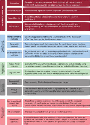
This article provides an overview of survival analysis in cardiovascular research and aims to provide a practical tool to understand the range of statistical approaches to tackle time-to-event outcomes. We briefly describe features of survival time data and provide an overview of several analytical approaches. For a better understanding, we will illustrate how these methods have been applied to data from cardiovascular studies. This review is primarily descriptive in content, and consequently no prerequisite mathematical, or statistical background are necessary. Basic concepts are summarized in figure 1.

Survival analyses are applicable when the measure of interest is time until the occurrence of an event (time-to-event outcomes). Despite using the word “survival”, the event or outcome can be fatal or nonfatal (eg, cardiovascular mortality or myocardial infarction, respectively).1 The time at which the event occurs is referred to as an event time, survival time, or failure time. The last 2 terms arose from the statistical methods developed for data analysis in cancer trials and for quality testing in manufacturing, respectively. Despite the term, the event under study is not necessarily a failure with negative connotations, meaning it could well be a positive event, such as appropriate implantable cardioverter defibrillator discharges.2
The survival time for each individual is the time from the starting point until the occurrence of the event of interest.1,3 In a randomized clinical trial (RCT), survival time is usually estimated from the randomization (usually occurring at the start of the intervention).4 In an observational study, survival time is more commonly calculated from entry into the study, from a particular fixed date, such as the date when participants are first exposed to a risk factor (eg, chemotherapy) or to an index event (eg, acute coronary syndrome [ACS]).5 Sometimes it is also calculated from an age point.
Sources of survival dataThere are 2 main sources of survival data in cardiovascular research: RCTs and observational studies.
In RTCs, the aim is usually to provide reliable evidence of treatment efficacy (or effectiveness), and safety. The simplest example involves individuals meeting the entry criteria, who are randomized to the intervention or the control group and followed up for a given time to collect events and time to events. For example, the REBOOT trial (NCT03596385) is randomizing patients with acute myocardial infarction and left ventricular ejection function ≥ 40% to receive either standard treatment with beta-blockers or not who will be followed up for a median period of 2.75 years to assess differences in the incidence of the composite endpoint of all-cause death, nonfatal reinfarction, or heart failure hospitalization.
In prospective observational studies (cohort studies), individuals differing in a primary exposure factor are recruited to a cohort and followed up for a range of different times, in order to compare time-to-event outcomes in those exposed and not exposed to the factor.6 The EPICOR (l Long-term follow-up of antithrombotic management patterns in acute coronary syndrome patients) registry is an international cohort study, which recruited postdischarged patients with an ACS who were followed up for 2 years for a variety of outcomes.7 Its entry time (time zero) was fixed at discharge after an index event (ACS), and the events collected over follow-up were other cardiovascular events (such a recurrent ACS) and fatal events. The EPICOR registry has been used to evaluate differences in all-cause mortality across a variety of exposures, such as the geographic origin of the participants,8,9 or whether they underwent coronary revascularization.5
In addition to RCTs and observational studies, other data sources for survival data that can be used, such as registries of administrative data. In Spain, the Spanish Minimum Data Set has been used to describe temporal trends and in-hospital complications of several cardiovascular conditions.10 However, their cross-sectional nature makes any time-to-event analysis impossible.
Features of survival data: uninformative censoringA key analytical problem in longitudinal studies (either RCTs or observational) is that the time to the event of interest may be censored, which means that for some participants the follow-up may not be complete and hence, the event is not observed to happen. There are generally 3 reasons why censoring may occur during the study period of a given RCT evaluating major adverse cardiac events (MACE): a) the event might not be recorded for patients who are still alive at the end of follow-up; b) participants lost to follow-up after a certain date (eg, migration); and c) those who died from a different cause (eg, cancer). In any of these situations, the actual survival time (eg, time to MACE) is unknown. It would be inappropriate to exclude such individuals from the analyses, since the fact that they did not experience MACE while they were in the study provides some information about survival. Of note, we only observe a time up to which we know they have not had the outcome at the “right side” of the follow-up period (a phenomenon known as right-censoring).1
The concept of censoring makes survival methods unique. For each patient we have 2 pieces of data: a) a time that is either the patient's event time, or the time at which the patient was last followed up; and b) an indicator that denotes whether the time is an event time or a censoring time. In other words, each patient has either an event time or a censoring time after which the patient would no longer be observed. It will be assumed throughout most of this review that censoring is uninformative about event times.1 This means that the time at which an individual is censored, or the fact that he or she is censored is not related to our time-to-event outcome. If a patient enrolled in an RCT drops out of the study, due to reasons related to the study (eg, participants in the intervention arm feeling better or having adverse effects) the censoring then becomes informative.
Violating this statistical assumption challenges the principles of the main approaches for survival data.11 Methods to address censoring due to a competing event (eg, death from another cause) will be discussed in our second review.
Key concepts in survival distributionsTwo relevant functions are needed to understand and describe survival distributions. The survival function, S(t), is defined as the probability that a person “survives” beyond any specified time (or t), whereas the hazard function, h(t), is defined as the instantaneous failure rate. The hazard function is a conditional failure rate (conditional to those who have survived until time t). For instance, in a study assessing MACE, the function at year 2 only applies to those who were event-free in year 2, and does not take into account those who had MACE before year 2. Note that, in contrast to the survival function, which focuses on not failing, the hazard function focuses on failing, that is, on the event occurring.
The hazard ratio (HR) is a measure of effect/association widely used in survival analyses. In its simplest form, the HR can be interpreted as the chance of an event occurring in the treatment arm (or exposed group) divided by the chance of the event occurring in the control arm (or unexposed group), of an RCT (or an observational study). The HR summarizes the relationship between the instantaneous hazards (or event rates) in the 2 groups. The HR is estimated using regression-type analyses.
Aims and approaches of survival analysesMost clinical studies focus on evaluating the impact of an intervention (eg, beta-blockers) or exposure (eg, geographic origin) on an outcome of interest (eg, MACE). In the setting of survival analyses, the outcome of interest is the survival time, and the focus is on either comparing survival times between treatment groups, or assessing the association between survival times and exposed vs nonexposed participants.
Methods for survival data need to account for censoring and the fact that survival times are strictly nonnegative and commonly skewed to the right. If censored observations were excluded from the analysis, the results would be biased, and the estimates would be unreliable. Three basic approaches are presented in this review:
Nonparametric methods. These relatively simple methods (eg, Kaplan-Meier estimates) do not make assumptions about the distribution of survival times. They are excellent for univariate analyses (eg, primary outcome in RCTs), but not sufficient to handle more complex problems, such as confounding in observational studies.
Fully parametric methods. These are regression-type analyses for survival data (eg, Weibull model), which are analogous to regression approaches for other types of response (eg, linear regression for continuous data, or logistic regression for a binary response). Nevertheless, they rely on some assumptions about the patterns of survival times, which should be carefully investigated.
Semiparametric methods. These lead to another regression-type analysis for survival data, often called Cox regression. The way survival times are associated with exposures of interest is parametrized, although they leave part of the full distribution of the survival times unspecified.
NONPARAMETRIC ANALYSIS OF SURVIVAL DATANonparametric techniques do not make any assumptions about the distribution of survival times, which makes sense since survival data have a skewed distribution. The most common nonparametric approach for modeling the survival function is the Kaplan-Meier estimate. This method uses the actual observed event and censoring times.
Why use nonparametric methods?Nonparametric methods are an appropriate starting point for most survival analyses. First, these methods allow estimation of survivor and hazard functions without the need to make parametric assumptions. Second, they provide a highly intuitive way of graphically displaying survival data, taking into account censoring data. Third, these techniques are optimal to compare survival time by groups of individuals (categorical variables). Finally, nonparametric methods can be used to provide information about whether some model assumptions can be made in more complex approaches of survival data (eg, proportional hazards assumption).
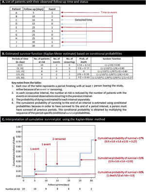
Estimating the survival function: the Kaplan-Meier methodThe simplest way to obtain an estimate of the survival function is by calculating the cumulative survival experienced by the participants included in a cohort. This can be achieved using the Kaplan-Meier method, which estimates the cumulative survival (and failure) probabilities every time a participant leaves the study. The Kaplan-Meier estimate is also known as the “product limit estimate”. This approach is based on conditional probabilities and is thoroughly explained in figure 2.
, whereas 5 patients have censored data: 4 patients are lost to follow-up (2 at day 15 and 2 at day 25), and only 1 patient finishes the follow-up without an event (censored at day 30). B: estimate of the survival function using the Kaplan-Meier method. C: interpretation of cumulative survival probabilities. As occurs with this example, the Kaplan-Meier survival estimate sometimes takes the form of a step plot rather than a smooth curve, reflecting the fact that this is an empirical estimate of the survival experience of a cohort at each time point. Importantly, censored observations do not reduce cumulative survival, but rather adjust the number at risk for when the next death occurs.")
How to build a Kaplan-Meier curve and estimate its survival function. A: in this example, we created a basic data set of 10 patients with a follow-up of 30 days. All of them are “at risk” of having the event at time 0. Five patients have the event (days 5, 10, 25, 25, and 30), whereas 5 patients have censored data: 4 patients are lost to follow-up (2 at day 15 and 2 at day 25), and only 1 patient finishes the follow-up without an event (censored at day 30). B: estimate of the survival function using the Kaplan-Meier method. C: interpretation of cumulative survival probabilities. As occurs with this example, the Kaplan-Meier survival estimate sometimes takes the form of a step plot rather than a smooth curve, reflecting the fact that this is an empirical estimate of the survival experience of a cohort at each time point. Importantly, censored observations do not reduce cumulative survival, but rather adjust the number at risk for when the next death occurs.
Another nonparametric approach is the life-table estimate of the survival function. For the Kaplan-Meier estimate, a discrete time setting is assumed (all survival times are observed at an exact time). Sometimes this piece of information is less precise and survival times are observed within a time range. A typical example is the evaluation of the number of deaths per year in a study population. In this setting, the life-table method is still popular in that it provides a simple summary of survival data in large study populations within time intervals.12
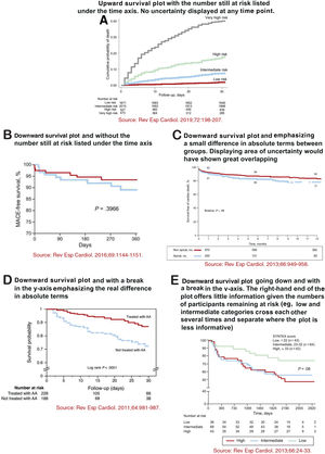
Recommendations for displaying Kaplan-Meier plotsKaplan-Meier plots are presented in almost all articles reporting survival analyses. Because of their prevalence, it is important to provide some suggestions for their appropriate representation. A poorly graphed Kaplan-Meier curve can lead to an erroneous interpretation by readers. In a landmark article published around 20 years ago, Pocock, Clayton and Altman examined the survival plots shown in 35 RCTs and suggested some key recommendations to consider when presenting Kaplan-Meier plots.3 In most cases, survival plots are best presented going upwards (cumulative proportion experiencing the event) rather than downwards (cumulative proportion free of the event). Usually, upward plots highlight relative differences, because the x-axis can be adapted to the scale of the curves. Instead, downward plots (using the whole vertical axis from 0 to 100%) make differences look much less pronounced and mainly emphasize differences in absolute terms. Therefore, a break in the y-axis should be avoided. Overlooking such a break may lead the reader to a mistaken perception of the potential treatment effect (or association), which would seem larger than the real difference. Ideally, plots should include some measure of statistical uncertainty—the standard error (or 95% confidence interval) for the estimated proportion of patients with (or without) the event can be calculated at any timepoint. In the rare cases when this uncertainty is presented, there is an increasing size of the standard error (or 95% confidence interval) bar over time, which illustrates the decreasing number of participants at risk in the follow-up. Finally, plots should extend in time as far as there are a sufficient number of participants in the study and the number of participants at risk remaining in the study should be shown below the x-axis. If there is a large decline in the number of participants during the course of the study, then caution should be exercised when interpreting differences between the curves in the right-hand side of the graph. These recommendations are illustrated in figure 3 with examples from articles published in Revista Española de Cardiología.13–17

A-E: 5 examples of different ways to display Kaplan-Meier curves. Reproduced with permission from Elsevier and Revista Española de Cardiología. The source of each plot is displayed below each Kaplan-Meier plot and full references are shown in the reference list.13–17 AA, aldosterone antagonist; MACE, major adverse cardiac events.
The log-rank test is used to compare the survival distributions of 2 or more groups. This nonparametric test, which only assumes the censoring to be noninformative, is based on a very simple idea: comparing observed vs expected events in each group. For the comparison of 2 groups (eg, testing the null hypothesis that the survival experience is the same for patients randomized to beta-blockers and control patients), we calculate the number of expected events in each group with the usual formula for 2x2 tables, for each time interval. The test will be carried out by comparting the sum of these “table-specific” expected values with the total observed events. If the observed numbers statistically differ from those expected, we may assume that the difference in the 2 groups is not happening at random. This approach can be also applied to explanatory variables with more than 2 groups, although the test statistic is more complex to calculate manually and its statistical power decreases as the number of comparisons increases.
Limitations of nonparametric methodsNonparametric methods for analyzing survival data are widely used, though they are not exempt from major limitations. They do not allow using continuous factors as dependent variables (it should be categorized to estimate hazards for people falling into different categories). Following the same reasoning, analyses involving several exposure variables, which may be binary continuous or categorical, are not possible unless each patient is categorized into a single category (eg, for 2 factors with 3 categories, there will be 6 groups). This approach usually ends with small groups limiting any formal comparison. Even more importantly, there is no way to adjust for potential confounders, but to look separately at groups defined by the confounder (hence these methods quickly become cumbersome and the groups too small for meaningful analysis). Taking all these limitations into account, a more advanced approach by using regression modeling can be applied to handle survival data.
PARAMETRIC REGRESSION MODELINGRegression modeling is about establishing a mathematical model for the survival times, which defines how survival times depend on individual exposures (or randomized allocations). It is analogous to the use of other regression-type analyses, such as linear regression to study the dependence of continuous response variables on explanatory variables, or logistic regression to study the dependence of a binary outcome on explanatory variables. Regression models for survival data can be parametric or semi-parametric18–20 and both provide a measure of effect known as HR. The models presented in this section are described as parametric, because they assume a particular shape for the distribution of the survival times which depends on defined parameters. In other words, survival times are assumed to follow a known distribution.
Why use parametric regression modeling for survival data?Choosing a theoretical distribution to approximate survival data is as much an art as a scientific task, and regression modeling is going to be always a simplistic way to summarize the reality. Parametric models assume that the survival and hazard functions have a specific distribution which is often too structured and sometimes unrealistic for use with real data.21 It is hard to isolate all potential causes that can lead to an event at a particular time, and to account mathematically for all of them. Nevertheless, there are some potential scenarios where it is appropriate to use parametric models.
The exponential modelThe most basic parametric model for survival time is the exponential distribution, which is a form of the survival distribution characterized by a constant hazard function. According to this model, having a failure (or event) is a random event independent of time. The exponential distribution, often referred to as a purely random failure pattern, is well-known for its “lack of memory” which means that a subject's probability of an event in the future is independent of how long the subject has gone without an event.1 The exponential distribution is characterized by having a single parameter (λ), a constant hazard rate. Hence, a high λ value indicates high risk and short survival, whereas a low λ value indicates low risk and long survival.18 Exponential models are rarely used in the cardiovascular field, but it has been applied in other areas, such as cancer22 or smoking cessation.23
The Weibull modelIn many scenarios, it would not be reasonable to assume a constant hazard rate over time,18 as under the exponential distribution. An alternative approach is to consider the Weibull distribution to parametrize survival times. Unlike the exponential distribution, it does not assume a constant hazard rate (hazard function is increasing or decreasing over time) and therefore has more flexibility, and a broader application. This method can be used when the hazard function in monotonically increasing or decreasing, and therefore is characterized by 2 parameters: the scale parameter λ (the same than for the exponential distribution), and the shape parameter γ, determining the shape of the distribution curve.24 By adding a shape parameter, the distribution becomes more flexible and can fit more types of data (with increasing, decreasing, or constant risk). A value of λ <1 indicates that the failure rate decreases over time, whereas if λ> 1 the failure rate increases with time. When the scale parameter (λ) equals 1, the failure rate is constant over time (Weibull reduces to an exponential model).
The reality about parametric regression modelingParametric regression models produce smooth predictions by assuming a functional form of the hazard and by directly estimating absolute and relative effects.24 In addition to the exponential and Weibull models, there are other parametric models (eg, Gompertz, Lognormal, etc.),18 but they fail beyond the scope of this review because the use of parametric modeling for survival data is relatively rare in cardiovascular research. Nevertheless, some recent examples can be found. In 2 recent publications from major RCTs, the Weibull regression model has been used to evaluate time to discontinuation to treatment allocation for informative reasons (eg, death).25,26 In the ENDURANCE trial, which compared a small centrifugal-flow left ventricular assist device to an axial-flow left ventricular assist device in patients with advanced heart failure who were ineligible for heart transplantation, the Weibull model was used for the primary endpoint of survival free from disabling stroke or device removal for malfunction or failure.27
THE COX PROPORTIONAL HAZARDS MODELThe Cox proportional hazards (CPH) model is the most popular approach to evaluate the relationship between covariates and survival 1,18 and was first proposed by Cox in 1972 to identify differences in survival due to treatment and prognostic factors in clinical trials.19,28 Whereas nonparametric methods typically study the survival function, with regression methods the focus is on hazard function.
The CPH is referred to as a semiparametric approach,28 as under this model the baseline hazard function is not parametrized, but the effect of the explanatory variables on the hazard is parametrized (using β coefficients). In other words, the baseline hazard is left unspecified (not written in terms of parameters to be estimated), which means that no assumptions are made regarding the baseline hazard function for each group (survival rates can vary between exposed and unexposed in an observational study, or intervention and control groups in a RCT1), whereas the ratio of their hazards is assumed to be constant. What is parametrized are the effects of the covariate variables upon survival, which are constant over time and additive in one scale. We can test the association of each of the independent variables with survival time adjusted for other covariates.
Model assumptionsLike any other statistical model, the CPH method relies on some assumptions. Nevertheless, the semiparametric approach makes fewer assumptions than the alternative parametric methods:
- •
The main assumption of the Cox model is that the HRs (defined as the ratio of the hazards between 2 groups) are independent of time. In other words, the ratio of hazards between groups is constant over time. This is known as the proportional hazards (PH) assumption. If an explanatory variable has a strong association with survival at the beginning of the follow-up but a weaker effect later on, this would be considered a violation of the PH assumption.
- •
The assumption that we have correctly specified the form of the explanatory variable – this assumption is bound to the PH assumption, since this may hold for a specific form of the explanatory variable but not for another. To comply with this assumption, explanatory variables might benefit from some transformation. Some continuous variables can be remodeled either using a binary cutoff point, for example for body mass index and hemoglobin, or using its continuous nature only above a certain threshold, for example for creatinine and blood glucose.29 The most common situation is the log transformation of highly skewed variables.
- •
Censoring is uninformative.
- •
Observations are independent.
Based on the above, the Cox model can fit any distribution of survival data if the PH assumption is valid (actually, most HRs are fixed proportional). For this reason, the Cox model is used so widely.
Model checkingBefore reporting any findings, we should check, as far as possible, that the fitted model is correctly specified. If not, our inferences could be invalid, and we may draw incorrect conclusions. Model checking is not an easy issue in survival analysis. In this section, the focus will be on assessing the PH assumption, though some methods for assessing whether the functional form for the explanatory variables is correct, are also provided. The last 2 assumptions are not formally testable.
There are 3 main ways of assessing whether the PH assumption can reasonably hold.30 The first of these methods involves the use of Kaplan-Meier estimates. If a categorical predictor satisfies the PH assumption, then the plot of the survival function vs the survival time will yield 2 parallel curves. Similarly, the graph of the log(-log[survival]) vs log of survival time graph should result in parallel lines if the predictor is proportional. This method becomes problematic with variables that have many categories and does not work well for continuous variables, unless they are categorized. Furthermore, the situation becomes too complex in multivariate models with several explanatory variables, which would need to be simultaneously tested using combinations of the covariates.31 Hence, this approach quickly becomes cumbersome and unrealistic for more than 2 or 3 variables. The second method to check for the PH assumption is by formally testing whether the effect of explanatory variables on the hazard changes over time (this can be done by including an interaction between time and the explanatory variable into the model). A significant interaction would imply the hazard function changes over time, and the PH model assumption would be violated. The third useful way to assess this assumption is through scaled Schoenfeld residual plots. Schoenfeld residuals can essentially be thought of as the observed minus the expected values of the covariates at each failure time.31,32 The plot of Schoenfeld residuals against time for any covariate should not show a time-dependent pattern.
In addition to checking for the PH assumption, other aspects of model fit can be assessed using residuals.30 Martingale residuals can be used as a way of investigating the appropriate functional form for continuous variables. A Martingale residual is the difference between what happened to a person (whether they had the event or not) and what is predicted to happen to a person under the model that has been fitted.33 A plot of the martingale residuals from a null model (model without explanatory variables) against a continuous variable can be used to indicate the appropriate functional form for the continuous variable when it is entered in the model. Deviance residuals and other approaches are beyond the scope of this review.
Final remarks about nonparametric, parametric, and semiparametric approachesKaplan-Meier plots are an excellent way of graphically illustrating the survival experience over time, particularly when the rate of the outcome changes irregularly. Should the exact survival or censoring time of each patient be known, the plots are easy to produce by researchers, and easy to interpret by readers. The log-rank test is a simple tool that provides a significance test for comparing survival times between groups. However, the log-rank test only provides a P value and does not provide a measure of effect, unlike any regression-type approach providing a HR. A further advantage of the HR approach (either parametric or semiparametric) is that it provides tools to investigate confounding and effect modification. Hence, nonparametric approaches are used to explore data and provide crude estimates, but regression-type approaches are commonly used to provide more precise estimates.
Developing an analysis strategy is a complex task. In survival analysis, incorporating model checking for PH assumption into our strategy adds an extra layer of complexity. This can be done at different points in the model building process. Nevertheless, if the PH assumption does not hold, some other options can be applied (changing the functional form of the explanatory variables entered in the model, using stratified CPH models, or using another type of approach that will be explained in the second part of this review).
STRATEGY OF ANALYSIS: SET OF RECOMMENDATIONS AND SUGGESTIONSDifferent strategies can be used in the setting of survival analyses. The approach to the data mostly depends on the type of study and the research question. In this section, we provide some suggestions for RCTs focused on estimating a treatment effect, and for observational studies focused on evaluating associations between exposures and survival times. These recommendations are not the only way to perform valid analyses—they are just a summary of a method covering all key aspects.
Randomized controlled trialIn a large RCT we can fairly assume that there are variables confounding the association between the randomized intervention and the outcome. One sensible strategy to evaluate survival data would be to: a) describe the numbers of participants in the allocation groups and summarize the number of events in each group; b) provide Kaplan-Meier estimates of the survivor curves in the treatment groups, and use the log-rank test to evaluate the alternative hypothesis (survivor curves differ between treatment groups); c) use plots to informally evaluate whether a PH model would be appropriate to yield a reliable estimate for the association between treatment and survival time (plots appear parallel when hazards for both groups are proportional); d) if a PH model seems reasonable, fit a CPH model (or a parametric model, if appropriate) to estimate the HR with its 95% confidence interval, and corresponding P value; and d) perform more formal assessments of the PH assumption (eg, by testing for an interaction of the treatment effect with time, or by plotting Schoenfeld residuals).
Observational studiesThe research question raised in an observational study determines the choice of explanatory variables to be used in a survival model. Sometimes the focus is on estimating an exposure “effect”—the interest is mainly in one particular exposure, but other variables are needed to control for potential confounding. On other occasions, the focus is on understanding the associations between a set of explanatory variables and the time-to-event. In this case, the interest is in the independent concomitant associations of several exposures on survival, perhaps to determine which has the greatest impact on survival. Strategies for addressing these 2 types of observational studies are presented in the next section.
Prediction modeling, where the aim is to use a set of variables to build a model to predict survival in individuals from a new cohort,34,35 is not covered in this review. In this setting, the term “predictor” is better suited than the term “explanatory variable”, and the strategy is focused on producing precise estimates for outcome prediction and assisting in risk stratification and clinical decision-making. Further details about prediction modeling can be found elsewhere.34,35
In the case of observational studies aiming to estimate an exposure “effect”, we suggest the following 3-step process based on a preliminary approach, a main analysis, and a final set of checks for modeling assumptions. Preliminary analyses would include: a) using Kaplan-Meier plots and log-rank tests to assess univariate associations between each exposure and the outcome; b) using nonparametric and residual plots to make preliminary assessments of the PH assumption for each exposure; and c) evaluating the association between the main exposure and each potential confounder by a simple but visual method (eg, using cross-tabulation). Assuming a PH model would be appropriate (either a parametric model, or most commonly a Cox model), the main analysis would therefore involve the following 7 steps: a) fitting a survival model using only the main exposure to estimate the univariate association; b) fitting further survival models using the main exposure and adding each potential confounder, one at a time; c) evaluating the impact of adjusting for each confounder on the estimated association between the main exposure and survival (eg, change in magnitude and direction of HR); d) assessing whether any covariate modifies the association between the main exposure and the event (eg, whether there are interactions); e) fitting a multivariate model for the main exposure, with adjustment for confounders (prespecified based on clinical knowledge, or found in step c and for interactions (found in step d); f) forcing those remaining potential confounders, not included in the model, back into the model one by one to evaluate whether they are confounders in the presence of other covariates; and g) adding any relevant confounders found in step f to the final model. Finally, further checks for modeling assumptions and overall model fit should be made before formally reporting the findings (eg, by testing for an interaction of the treatment effect with time, or by plotting Schoenfeld residuals of the final model).
In a situation without a clear prior hypothesis about which explanatory variables may be associated with survival, sometimes it may be necessary to perform an exploratory analysis. If there are not too many variables, it would be sensible to include them all in a model and evaluate the associations between each variable and the outcome after full adjustment for all other covariates. Alternatively, a similar 3-step process, based on a preliminary approach, a main analysis, and a model check, would be useful. Preliminary analyses would include using Kaplan-Meier plots and log-rank tests to evaluate the association between each variable and the outcome. After this first approach, the main analysis needs to address the issue of selecting the “best” set of covariates. This approach would require the following tasks: a) evaluating each variable separately in a sequence of PH models (Cox or parametric, when appropriate) in order to assess univariate associations between explanatory variables and the outcome; b) including all variables selected in the previous step in a single PH model, and then excluding each variable one by one, to assess whether the exclusion has a significant impact on the log likelihood (statistical significance can be tested using likelihood ratio tests); c) entering each of the variables that have been removed in the previous step back into the model one by one, to check whether they add anything to the model (using likelihood ratio tests), and d) repeating step c as many times as needed for all explanatory variables that remain out of the model in each “cycle”. Finally, further checks on modeling assumptions should be performed, as explained for other types of analyses.
Other approaches for the latter 2 scenarios would be to use automatic tools to select explanatory variables, such as forward or backward selection step processes. Although they are valid in some scenarios (particularly prediction modeling), one should bear in mind that regression modeling is as much an art as a scientific task, which requires medical knowledge, as well as statistical expertise and experience.
CONCLUSIONSThis is the first in a series of 2 educational articles reviewing the basic concepts of survival analyses, laying the foundations to understand, compare and apply the most relevant statistical models for survival analyses. Aiming to reach readers without much background in statistics, a key feature of this review is the integration of the essentials of survival analysis with practical examples from cardiovascular studies, showing the reader how to perform survival analyses and how to interpret their results. The main model assumptions are presented to provide the tools to apply the appropriate statistical model according to the shape of the data. Additionally, recommendations to guide the strategy of analyses have also been provided, in the hope that they might have an impact on the critical appraisal and statistical performance of readers. The second article will tackle a variety of more complex statistical challenges that are often faced in survival analyses. These include competing risks, recurrent-event methods, multistate models, and the use of restricted mean survival time.
FUNDINGNone.
AUTHORS’ CONTRIBUTIONSX. Rossello and M. González-Del-Hoyo conceived the review. X. Rossello led the writing process, and M. González-Del-Hoyo was in charge of finding most of the examples to illustrate the methods. X. Rossello drafted the article, though both authors contributed substantially to its revision.
CONFLICTS OF INTERESTNone declared.