This article is the second of a series of 2 educational articles. In the first article, we described the basic concepts of survival analysis, summarizing the common statistical methods and providing a set of recommendations to guide the strategy of survival analyses in randomized clinical trials and observational studies. Here, we introduce stratified Cox models and frailty models, as well as the immortal time bias arising from a poor assessment of time-dependent variables. To address the issue of multiplicity of outcomes, we provide several modelling strategies to deal with other types of time-to-event data analyses, such as competing risks, multistate models, and recurrent-event methods. This review is illustrated with examples from previous cardiovascular research publications, and each statistical method is discussed alongside its main strengths and limitations. Finally, we provide some general observations about alternative statistical methods with less restrictive assumptions, such as the win ratio method, the restrictive mean survival time, and accelerated failure time model.
Keywords
Based on the fundamentals covered in the previous review article,1 this second paper explores more complex challenging situations in survival analyses. We now present some extensions to the Cox proportional hazards (CPH) model, such as the stratified and frailty models, and the use of time-dependent variables. We explore the problems faced by researchers in the cardiovascular field due to multiplicity of outcomes, and present some approaches to tackle this issue, such as the use of composite outcomes, competing risks, multistate models, and recurrent-event methods. An increasingly popular topic is the use of the win ratio approach. To provide a comprehensive overview of the most common statistical approaches in survival analyses, some other methods are briefly introduced, such as the restrictive mean survival time, and accelerated failure time model approaches. For a better understanding, we will illustrate how these methods have been applied to data from cardiovascular studies. This review is primarily descriptive in content, and therefore no prerequisite mathematical or statistical knowledge is necessary.
EXTENSIONS OF THE COX PROPORTIONAL HAZARDS MODELStratified Cox proportional hazards modelThe CPH model is by far the most commonly used model in survival analysis. Some extensions to this model can be considered when it does not provide a good fit to our data. In the stratified CPH model, instead of assuming that the proportional hazards (PH) model holds for the overall cohort, we assume that the PH model holds within groups (or strata) of individuals. Study variables that are assumed to satisfy the PH assumption are included in the model, whereas the factor being stratified is not included, and is controlled by stratification. Hence, this method does not provide an estimate of the effect of the factor (or factors) defining the groups on the hazard (ie, it does not provide a hazard ratio of the stratifying variable) and is therefore not a suitable approach if the factor exhibiting nonproportionality is of primary interest. To evaluate the effect of mineralocorticoid receptor antagonists in preventing sudden cardiac death in patients with heart failure (HF) with reduced ejection fraction, a stratified CPH model was needed to address the inevitable baseline differences across 11 032 patients recruited from 3 placebo-controlled randomized trials (RCTs): RALES (Randomized Aldactone Evaluation Study), EPHESUS (Eplerenone Post–Acute Myocardial Infarction Heart Failure Efficacy and Survival Study), and EMPHASIS-HF (NCT00232180). Although all patients had in common the fact that they had HF with reduced ejection fraction, participants from EMPHASIS-HF were in New York Heart Association class II, whereas those from RALES were in New York Heart Association class III-IV, and participants from EPHESUS had a recent myocardial infarction (MI).2 In other cases, CPH models are stratified by geographic region and baseline renal function at baseline.3
Frailty modelsIn a stratified CPH, baseline hazards functions from different strata are unrelated. This is based on the assumption that the study population is homogeneous across strata. However, individuals may differ greatly within strata (eg, in an RCT, with respect to the treatment effect, whereas in an observational study, with respect to the influence of covariates in a given association). The presence of unobserved individual-specific risk factors leads to unobserved heterogeneity in the hazard, which is also referred to as frailty, or a random effect. Importantly, in many situations the population cannot be assumed to be homogeneous (eg, a mixture of participants with different hazards). In this case, in contrast to the CPH model, a frailty model is useful as it implies that baseline hazard functions are proportional to each other.
Frailty models are random effects models for time-to-event data,4 in which the random effect has a multiplicative effect on the baseline hazard function. In the context of survival models, this random effect is called “frailty” for historical reasons, as the term simply refers to the fact that some individuals are intrinsically more “frail” than others. The classic example occurs when a study involves the recruitment of patients from different hospitals. Survival times from participants at the same hospital tend to be similar (eg, due to treatment practices, level of tertiary activity, etc) and there is a greater between-hospital variability than within-hospital variability. These clustered (or hierarchical) data need a model accounting for the clustering. A natural way to model dependence of clustered event times is through the introduction of a cluster-specific random effect—the frailty.4 This random effect explains the dependence in the sense that had we know the frailty, the events would be independent. The use of frailty models is relatively popular. They have been applied in some studies using the EPICOR (Long-term Follow-up of Antithrombotic Management Patterns in Acute Coronary Syndrome Patients) registry,5 where in addition to adjusting for age, sex and other relevant confounders, the model had a random effect (shared frailty) at the hospital level.5
Time-dependent variablesSometimes explanatory variables change over time in an individual (eg, treatment, blood pressure, or smoking status). These variables are known as time-dependent, time-updated, or time-varying variables. If changes over time in these variables are not taken into account, the results yielded by a survival model may provide a bias known as “immortal time” bias, or survivorship bias.6
Immortal time refers to a period of follow-up where the event of interest cannot occur because the subject has not yet started the exposure.6 A subject is not literally immortal during this period, but remains event-free until classified as exposed. An incorrect consideration of this unexposed time period in the analysis will lead to immortal time bias.6 If the unexposed follow-up time is misclassified as exposed, patients in the exposed group are inherently given a survival advantage. Consequently, immortal time bias of this type results in spurious protective effects of the exposure. Classic immortal time bias examples in the literature have been found in the Texas7 and Stanford Heart Transplant data,8 with both studies concluding that a heart transplant prolongs survival in those patients on a transplant waiting list. However, data were poorly analyzed because heart transplant was not treated as a time-varying variable. The waiting time of all patients who were alive until they received a transplant was classified as exposed to transplant (instead of unexposed), and gave a survival advantage time to the transplanted group. Deaths that occurred while waiting for a transplant were categorized into the nontransplant cohort. By not being correctly classified, the immortal time increased the mortality rate of the nontransplant group, suggesting a benefit of transplant.9 However, when adequately analyzed, the major survival advantage of the intervention disappeared when the follow-up times where properly accounted for.10
When estimating the effect of time-dependent covariates, the follow-up period has to be divided into subintervals (time until exposure and time from exposure onwards), which means that a subject might have more than one subinterval (eg, more than one row in the dataset, one for each subinterval). Subjects enter the study alive, awaiting the exposure, then are censored when they become exposed, and start a new subinterval of time (new row in the dataset) where the entry time is the censored time from the first subinterval, with a new covariate value indicating postexposure. Using the EPICOR cohort, Bueno et al.11 evaluated the impact of dual antiplatelet therapy (DAPT) duration in acute coronary syndrome patients, and the change from DAPT to single antiplatelet therapy (SAPT) in mortality. DAPT was entered into the model as a time-updated categorical variable (0 meant being on DAPT, 1 meant a change to SAPT). For patients who were always on DAPT, never receiving SAPT, the value of the time-updated variables was 0 throughout their follow-up. For those changing from DAPT to SAPT (usually after 1-year of follow-up), the authors provided follow-up time to both groups (time exposed to DAPT, and time exposed to SAPT).
Two approaches can be used to estimate the impact of time-dependent covariates12: the CPH model, which can accommodate time-dependent variables, and the landmarking approach. The latter involves setting a landmark time point and using the value of the time-dependent covariate at this landmark point as a time-fixed covariate. By using this approach, participants with an event before the landmark time point are excluded from the survival analysis, which starts from the landmark time point onwards, in the subset of participants at risk at that given time.
ALTERNATIVE MODELS FOR SURVIVAL DATAThe CPH model is the most common approach used for the analysis of time-to-event data. However, this regression model may not be appropriate in some situations, such as when the hazard ratio is not constant over time.13,14 Furthermore, one limitation of the CPH is that the hazard ratio is a relative measure that does not quantify absolute effects or associations. Other approaches may overcome some of the limitations of PH analysis. However, when PH are satisfied, the CPH model is the most statistically powerful method.13
Restricted mean survival timeRestricted mean survival time (RMST) is a measure of average survival from time 0 to a specified time point, and may be estimated as the area under the survival curve up to that point.13,14 Associations are expressed as the difference in RMST between groups at a suitable follow-up time, which is easy to interpret by both clinicians and patients (eg, if the outcome of interest is mortality, the estimate would be loss of life expectancy). In addition, the difference between RMST provides an absolute measure (eg, in a 2-arm RCT, RMST provides the absolute benefit or harm). This approach does not require assumptions about hazards and has the advantage of being valid under any distribution of survival time, or when it is expected for an association to vary over time, such as an intervention with either early or late treatment effects.
RMST analysis captures the entire survival history, does not change with extended follow-up time, and is routinely associated with a clinically meaningful time point.15 In HF RCTs, RMST seems to add value to traditional PH analyses by providing clinically relevant estimates of treatment effects, in line with the findings yielded by other statistical methods.16
Accelerated failure timeThis approach is known as the accelerated failure time model because the term “failure” indicates the death or event, while the term “accelerated” indicates the factor for which the rate of failure is increased. That factor is called the “acceleration factor”.17 Instead of the hazard, the key measure of the association between the study variable and survival time is the acceleration factor, which is a ratio of survival times. Similar to the CPH model, the accelerated failure time model describes the relationship between survival probabilities and a set of covariates, estimating a relative (not an absolute) association. The accelerated failure time model provides an estimate of the ratio of the median event times, which can be translated to clinicians as the expected reduction in the duration of illness with treatment.17
MULTIPLICITY OF OUTCOMES IN SURVIVAL ANALYSISClinical studies may evaluate multiple outcomes to try to maximize the information provided by clinical studies. In the field of cardiovascular research, the outcomes of interest might include stroke, HF, MI, sudden death, cardiovascular death, or all-cause death. To avoid inflation of the type I error rate by testing each outcome separately, a potential solution is to use a composite endpoint by including all the outcomes based on the time-to-first-event principle. Composite outcomes have several advantages,18 such as accounting for both fatal and nonfatal events, and hence leading to higher event rates and power (thus requiring smaller sample sizes or shorter follow-ups).19 Nevertheless, they also have some weaknesses,20 such as the underlying assumption that each individual outcome involved in a composite is of similar importance to patients.21 It is also common to have higher event rates and larger treatment effects associated with less important components.22 Hence, the use of composite outcomes is not always optimal. There are some situations that require more sophisticated statistical approaches than simply using a composite outcome on a time-to-first event basis, such as: a) the use of a competing risk assessment in the evaluation of nonfatal events, where the occurrence of fatal events can bias the findings; b) the use of multistate models to take into account intermediate states (eg, a HF hospitalization is common before an HF-related death)23; c) the use of recurrent-event methods to fully capture the burden of chronic diseases, which may involve several hospitalizations over the follow-up period; and d) the win ratio approach to provide a hierarchical assessment of the individual components of a composite outcome.
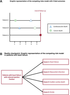
COMPETING RISKSThe censoring assumptionUninformative or independent censoring is assumed for the most popular approaches in survival analyses: those who are censored have the same hazard of the event of interest as those who are not censored.24,25 In other words, the uncensored individuals who remain under follow-up should be representative of the survival experience in the censored individuals. However, if censoring occurs due to another known event taking place, the assumption of uninformative censoring is violated. Competing risks occur when the event of interest is a particular cause of failure (eg, cardiovascular death), which can take place alongside other causes of failure (eg, noncardiovascular death due to cancer). The competing risk may prevent the event of interest from taking place: a person who dies of cancer is no longer at risk of cardiovascular death (figure 1).
Competing risk bias: impact on the cumulative incidence of events
A competing risk bias happens when censoring is informative due to multiple causes of failure. This bias has been reported in almost half of Kaplan-Meier analyses published in medical journals.26 If we estimate the survival probability of sudden death in patients with HF with reduced ejection fraction and censor the other causes of death (eg, HF-related death), the cumulative incidence of events over time (which is 1 minus the survival probability) will overestimate the probability of death due to sudden death.2 Indeed, by using the Kaplan-Meier estimator and censoring the other causes of death, we assume that those censored due to an HF-related death have the same future hazard of sudden death as those who have not yet had any event. Since those who have already died from other reasons can never experience death from sudden death, this can never be true. By assuming that those already dead from other causes are still at risk of sudden death, and that they can be represented by those not yet experiencing any event, the Kaplan-Meier approach overestimates the probability of failure, and therefore underestimates the probability of surviving at a given time. Another classic example, for patients with implanted cardioverter-defibrillators, can be found elsewhere.27
Addressing statistical analysis in competing risksTwo different hazard regression models are available in scenarios where competing risks are present28,29: modelling the cause-specific hazard, or the subdistribution hazard function.
A) The cause-specific hazard function (use of cumulative incidence function [CIF]). The CIF estimates the incidence of an event of interest while allowing for a competing risk. Individuals experiencing the competing event are no longer considered at risk of the event of interest. In the simplest case, when there is only 1 event of interest and no competing risks, the CIF would equal the 1–Kaplan-Meier estimate. The CIF takes into account both the probability of experiencing the event of interest, conditioned upon not experiencing either event (primary or competing) until that time. The sum of the CIF estimates for each outcome individually equals the CIF estimate of the composite outcome consisting of all competing events. Unlike the survival function in the absence of competing risks, the CIF function of the event of interest will not necessarily approach unity with time, because of the occurrence of competing events that preclude the occurrence of the event of interest.28 The CIF can be interpreted as the instantaneous rate of the primary event in those participants who are currently event free.
B) Fine and Gray model (use of subdistribution hazard function). Fine and Gray modified the CPH model to allow for the presence of competing risks.30 The subdistribution hazard function for a given type of event is defined as the instantaneous rate of occurrence of the given type of event in participants who have not yet experienced an event of that type. Hence, in this model, we are considering the rate of the event in those participants who are either currently event-free or who have previously experienced a competing event (although it feels unnatural to keep dead participants at risk for other events). This differs from the risk set for the cause-specific hazard function, which only includes those who are currently event free. In this way, there is a subdistribution hazard function for each outcome (eg, one for sudden death, and another for HF-related death).
The CIF model estimates the impact of covariates on the cause-specific hazard function, while the Fine-Gray subdistribution hazard model estimates the impact of covariates on the subdistribution hazard function.27 Because the CIF model relies on participants actually at risk (event-free participants), hazard ratios from this model should be interpreted among individuals who have not yet experienced the event of interest or the competing event and therefore this approach is optimal for answering etiological research questions. In contrast, by keeping at risk those individuals who have experienced the competing risk, the subdistribution hazard model may be of greater interest if the focus is on the overall impact of covariates on the incidence of the event of interest, and is optimal to perform risk prediction and risk-scoring systems.31
MULTISTATE MODELSDefinition of absorbing and nonabsorbing eventsAn absorbing event prevents the outcome of interest from subsequently taking place (eg, a cardiovascular death prevents a cancer death). Sometimes, there is an intermediate event, which may occur before the absorbing event, known as nonabsorbing event. These intermediate events are of particular interest when their occurrence substantially changes the likelihood of the outcome of interest happening, and hence, may provide more detailed information on the natural history of the disease. The intermediate event can be interpreted as a deterioration or improvement step in the disease process. This step was illustrated by Solomon et al.,23 who assessed the influence of nonfatal hospitalizations for HF on subsequent mortality in patients with chronic HF. In contrast to the relatively stable mortality risk observed over time in patients with HF from the CHARM (Candesartan in Heart failure: Assessment of Reduction in Mortality and morbidity) program, these authors found a higher likelihood of dying in the immediate post discharge period of a HF hospitalization, which was directly associated with the duration and frequency of HF hospitalizations.23 Having a HF hospitalization (nonabsorbing event) changed the hazard of the outcome of interest (mortality).
Nonabsorbing events can be modelled using multistate models,32 in which the focus is on the change of status over time (eg, change from baseline status to HF hospitalization, and from there to cardiovascular death).33
Multistate models: an extension of competing risks modelsMultistate models provide a framework that allows analysis of the natural history of a disease. These models are an extension of competing risks models (multistate model with 1 initial state and several mutually exclusive absorbing states), since they extend the analysis to what happens after the intermediate event.34 This review will consider only continuous time models allowing changes of state at any time. These models are more realistic and can be seen as an extension of the standard survival model, as they describe how an individual moves between a series of discrete states in continuous time.
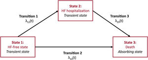
Multistate models are appropriate when a disease involves transitions between several well-defined distinct states. A 2-state survival model is defined by a living state and a dead state. The 2 main features of the standard survival model are: a) there is 1event of interest (the transition from alive to dead), which is unidirectional; and b) the timing of this event may be right-censored, in which case it is known that the event has not happened yet. A Kaplan-Meier curve can be thought of as a simple multistate model with 2 states, and 1 transition between those 2 states. The situation becomes more complex when nonabsorbing events are included in the model. In the HF setting, HF hospitalization can be defined as a transient event (nonabsorbing event). A 3-state survival model would be defined by a HF-free state, an HF state, and a dead state. This sets 3 events: death from state 1 (HF-free state), death from state 2 (HF state), and transition from state HF-free to HF hospitalization (figure 2). The hazard rates defining movement from one state to another are defined as transition intensities, the instantaneous risk of moving from one state to another at a given time. These transition intensities are equivalent to the cause-specific hazards described for the competing risks approach, this situation being a particular case of multistate models. There are as many hazards to model as there are transitions.
. HF, heart failure.")
To run a multistate model, a counting process data structure is used to frame the data. Hence, each time there is a transition, another row of information for that individual is needed in the dataset. In contrast, in a traditional time-to-first event survival analysis, there is only 1 row of information per patient in the dataset, including the status and the survival time (time-to-event or time to censoring).
Recurrence of nonfatal HF or MI are nonabsorbing events depending on time. Although they can be taken into account in standard survival models by including the nonabsorbing event as a binary time-dependent covariate for the risk of death, the best approach to tackle these patients’ transitions in various states is by multistate modelling.35 To improve understanding of prognosis, a comprehensive model should include both death and nonfatal clinical events. CPH models are not strictly appropriate since observations are not independent. Multistate models overcome this limitation by separately assessing time-to-death and time-to-disease-related hospitalizations.36
Multistate models in cardiologySeveral studies have used multistate models in the field of cardiovascular research.37 Beyond the classic example of chronic HF,36 we can find other examples in patients with multivessel coronary disease. Using data from the BARI trial (NCT00000462), Zhang et al.38 performed a multistate model, where the initial state was patients after randomization and before intervention, the intermediate state was nonfatal MI, and the final state was death. Standard survival analyses with Cox regression and Kaplan-Meier estimation for both mortality and the composite outcome of death or nonfatal MI showed no differences between coronary artery bypass grafting and percutaneous coronary angioplasty after a 10-year follow-up. Of note, this approach did not take into account the intermediate state (nonfatal MI). In contrast, multistate modelling broke the process into 3 transitions, and found significant differences in outcomes favoring coronary artery bypass grafting for patients in a transition path of nonfatal MI to death, whereas for patients without MI, there was no difference in terms of survival between patients who underwent coronary artery bypass grafting and those who underwent percutaneous coronary angioplasty. This study illustrates that the use of composite outcomes may not capture as much prognostic information as the use of a multistate model.
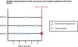
RECURRENT-EVENT METHODSDefinition of recurrent eventMost studies evaluate time-to-first event endpoints, so that all subsequent equal events occurring after a first one are ignored in the analysis. In HF, this problem becomes even more important as “time-to-first” event analyses do not fully reflect the true burden of the disease39: In patients admitted to Spanish emergency departments due to acute HF, 24% revisited the emergency department within 30 days, and 16% were rehospitalized in the same follow-up period.40 Of note, each subsequent HF hospitalization heralds a substantial worsening of the long-term prognosis.41 In contrast to conventional methods, the use of recurrent-event methods may capture the burden of disease (figure 3).
, patient B is hospitalized twice before dying (only the first hospitalization would be taken into account using traditional methods), and patient C dies during follow-up without any previous hospitalizations (using a composite endpoint, information about the disease burden would be lost in this situation).")
Graphical representation of the recurrent-risks model. Several situations in the context of recurrent events are illustrated: patient A is hospitalized 4 times during follow-up (only the first event would be used in conventional survival analyses), patient B is hospitalized twice before dying (only the first hospitalization would be taken into account using traditional methods), and patient C dies during follow-up without any previous hospitalizations (using a composite endpoint, information about the disease burden would be lost in this situation).
Recurrent-event methods have been generally assumed to improve statistical precision and provide greater statistical power than more conventional time-to-first methods. For instance, in the CHARM-Preserved trial,42 a borderline result for time-to-first composite event analysis was achieved. However, post hoc analyses with a recurrent-event method led to a gain in statistical power and showed significant evidence of efficacy.19
Statistical analysis in recurrent-event methodsThere are several statistical methods addressing the issue of recurrent events, but there is some controversy as to which of them is the most appropriate. There are 2 main approaches: through counts (or event rates), and through times between subsequent events. Noninformative censoring is assumed in both cases.
For the first approach, based on measuring the number of events (eg, number of hospitalizations due to worsening HF), there are 2 main methods.43 The Poisson distribution is the most popular count model and can be used to determine if event rates differ between groups, whereas the negative binomial distribution is an alternative approach that allows for different individual tendencies (frailties). The latter has been retrospectively used to evaluate recurrent hospitalizations in the EMPHASIS-HF trial.44 In the TOPCAT (NCT00094302) trial, the prespecified Poisson regression model was eventually replaced with a negative binomial model to allow for correlated events.45
There are many methods for the second approach, based on the time-to-event principle. The Andersen–Gill approach is an extension of the CPH model, which analyses recurrent events as gap times (eg, the times between consecutive events).46 The Lin-Wei-Yang-Ying method is a modified Anderson-Gill model, with a robust variance estimator to account for the correlation between events, which is useful when covariates are considered time dependent. This approach was used for the primary outcome of total (first and recurrent) HF hospitalizations and cardiovascular deaths in the PARAGON-HF trial.47 The Ghosh and Lin method offers a nonparametric estimate of the cumulative number of recurrent events through time, which incorporates death as a competing risk.48
Final remarks about recurrent-event methodsRecurrent-event models seem to improve statistical precision and to provide greater statistical power than time-to-first event approaches.49 However, the relative width of the 95% confidence intervals associated with recurrent-event analyses can sometimes be greater than that from time-to-first event analyses, suggesting a loss of precision.19 Using trial-based data (CHARM, TOPCAT, PARADIGM-HF [NCT01035255]), Clagget et al. found that the increasing heterogeneity of patient risk, a parameter not included in conventional power and sample size formulae, might explain the differences between time-to-first and recurrent-event analyses in terms of treatment effect estimation, precision, and statistical power.49 In that study, they concluded that the greatest statistical gains from using recurrent-event methods occur in the presence of high patient heterogeneity and low rates of study drug discontinuation.49
THE WIN RATIO METHODThe win ratio was introduced in 2012 by Pocock et al.50 as a new method for examining composite endpoints, and it is becoming progressively popular in cardiovascular RCTs.51,52 Unlike traditional methods evaluating composite endpoints, the win ratio accounts for relative priorities of their components, and even allows different types of components. For example, the win ratio can combine the time to death with the number of occurrences of a nonfatal outcome such as cardiovascular-related hospitalizations (CVHs) in a single hierarchical composite endpoint. It can also include quantitative outcomes such as quality-of-life scores.
Based on the principle of the Finkelstein-Schoenfeld test, the win ratio approach provides an estimate of the treatment effect (the win ratio) and confidence interval, in addition to a P value.53 In a simple 2-arm RCT, the application of the win ratio can be summarized as: a) forming every possible patient-to-patient pair (each patient in the treatment arm is compared with each patient in the control arm); and b) within each pair, evaluating the component outcomes in descending order of importance until one of the pair shows a better outcome than the other. If the patient on the treatment has the better outcome it is called a “win”, if the control patient does better it is called a “loss”, and, if none of these situations happens, then it is a “tie”.
This approach was used in the ATTR-ACT trial,52 which was a double-blind trial that randomized 441 patients with transthyretin amyloid cardiomyopathy to tafamidis (80 and 20mg), or matching placebo for 30 months. In the primary analysis, the investigators hierarchically assessed all-cause mortality, followed by the frequency of CVHs using the Finkelstein-Schoenfeld53 and win ratio50 methods. For each pair, they determined whether the patient receiving tafamidis “won” or “lost” compared with the patient receiving placebo. Their hierarchical assessment was to determine: a) who died first (the “loser”); and then, b) if neither died, who had the most CVHs (again the “loser”), both being assessed over their shared follow-up time. After adding up, they obtained a total of 8595 winners and 5071 losers. Hence, the win ratio was 8595/5071 = 1.70, with a 95% confidence interval of 1.26-2.29 and P = .0006.54 By using traditional methods to evaluate a composite outcome of first CVH or death, we would have ignored repeat CVHs after the first CVH, as well as any death happening after a CVH. The win ratio provides greater statistical power to estimate treatment differences by evaluating hierarchically each component of a composite outcome.
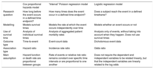
OTHER APPROACHES: LOGISTIC AND POISSON REGRESSION MODELLINGIn addition to CPH models, survival data is often evaluated using logistic and Poisson regression models.55,56 The choice between these models is based on the study design and the nature of the research question.57Table 1 summarizes the main differences between these models in the setting of survival analysis.
Summary of differences between the Cox proportional hazards, Poisson and logistic regression models
| Cox proportional hazards model | “Interval” Poisson regression model | Logistic regression model | |
|---|---|---|---|
| Research question | How long before the event occurs in a defined time endpoint? | How many times does the event occur in a defined time endpoint? | Does a subject reach the event in a defined timeframe? |
| Modelling | Models survival times | Models the rate at which the event occurs independently over time | Models whether an event occurs or not |
| Use of survival time | Analysis of individual survival times | Analysis of aggregated patient mortality rates | Analysis only of events, without taking into account when they happen. Does not use survival times |
| Outcome type | Time-to-event | Event-count data | Dichotomous event data |
| Association type | Hazard ratio | Incidence rate ratio | Odds ratio |
| Main assumption | Hazard function or death rate are proportional between groups | Rate of events or relative risk ratio remains constant over specific time intervals or are proportional to one another | Does not require the dependent and independent variables to be related linearly, but that the independent variables are linearly related to the log odds |
In this second educational review, we have focused on stratified CPH models, frailty models, and time-dependent variables. Competing risks, multistate models, recurrent-event methods and the win ratio approach have been presented to tackle the issue of multiplicity of outcomes when the use of a composite outcome and a time-to-first event might not be optimal. The use of restrictive mean survival time and accelerated time model approaches have also been illustrated. Adequately modelling survival data is not a straightforward exercise. This review has offered practical advice on what should be considered before choosing the most appropriate model for survival data, as well as some guidance to interpret the findings yielded by more complex statistical approaches.
FUNDINGNone declared.
AUTHORS’ CONTRIBUTIONSX. Rossello and M. González-Del-Hoyo conceived the review. X. Rossello led the writing process, and M. González-Del-Hoyo was in charge of finding most of the examples to illustrate the methods. X. Rossello drafted the article, although both authors contributed substantially to its revision.
CONFLICTS OF INTERESTNone declared.